Force Concentration: Lanchester and Trafalgar

Share this article:

One of the cornerstones of military thought is the concept of force concentration – focusing a large portion of one’s own fighting strength on a small portion of the enemy’s. With different wordings (American doctrine, for one, refers to it as mass) this maxim is present in the Principles of War followed by all modern armed forces, and we can find various expressions of it as far back as Sun Tzu’s time.

The principle of concentration might seem self-evident to us at first. It does not take a great deal of analysis to realise that having a superior force is an advantage in any armed conflict – it could even strike us as tautological, in that any force that wins a battle is automatically proving to be superior to its adversary.

In practice, however, it is all much subtler. To begin with, “superior force” can mean a number of different things, from a strictly numerical advantage to better training or equipment. Even more important is the idea that this superiority, whatever we take it to mean, does not need to happen everywhere at once. A force that is generally inferior might, through planning and manoeuvre, obtain superiority at a specific place and time in order to achieve an objective of military value. Quoting Air Marshal David Evans:

Concentration does not just mean a massing of forces. It implies having forces so disposed as to be able to unite to deliver the decisive blow when and where required, or to counter the enemy’s threats or attacks.

Evans, David – War: a Matter of Principles  (2000)

In other words, overwhelming the enemy is not exclusively a matter of numbers, but a consequence of being in the right place at the right time. To achieve success, a commander must strive to apply combat power when and where it is useful, while trying to avoid any engagement that is not favourable, or simply does not contribute towards a worthwhile purpose.

ANALYTICAL STUDY OF CONCENTRATION

When Frederick W. Lanchester presented his Square Law in his 1916 book Aircraft in Warfare, he envisioned it as a mathematical analysis of the principle of concentration . The same intention promoted the earlier (but classified until much later) work by J. V. Chase in 1902.

Arguably the best known mathematical combat model ever formulated, the Square Law is a set of two differential equations created to calculate attrition rates of two opposing forces, assuming all elements of force A can fire upon all elements of force B, and vice versa. They take the form:

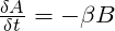
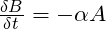
Where A and B are the number of elements in each force, and α and ß, known as Lanchester coefficients, are the number of enemy elements that A and B (respectively) can put out of action in a time increment.

Combining both equations, we see that two opposing forces will be exactly equal in fighting strength (and hence would eventually destroy each other if neither retreated) if the following equality is met:

The last expression shows that, under these assumptions, a force’s fighting strength scales with the square of its numbers – and for that reason we refer to it as the Square Law.

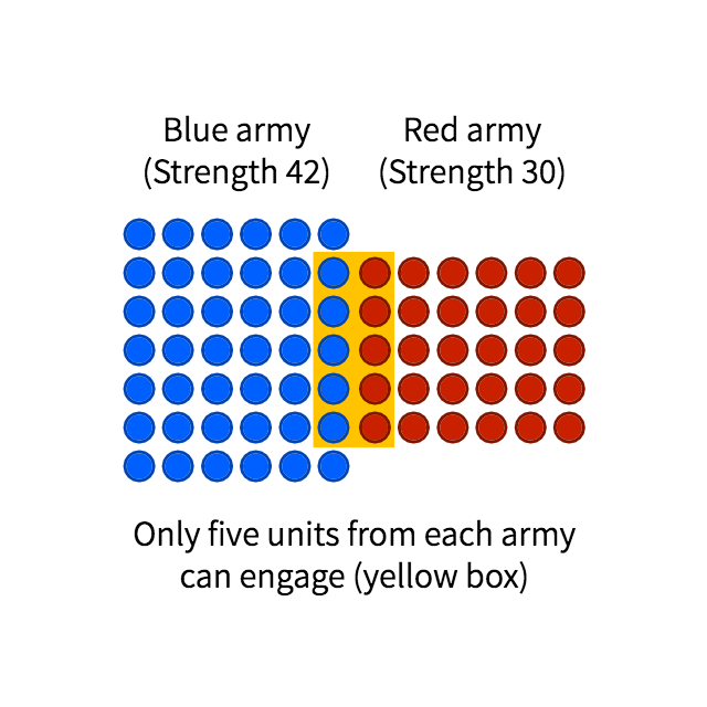
This conclusion is very often misunderstood as a statement that numerical superiority trumps all. Lanchester never believed so – how could he? Even a cursory glance at military history tells us otherwise. The truth of the matter is that a battle is never as simple as two forces uniformly inflicting casualties on each other over a period of time. Instead, we should look at it as a combination of smaller, discrete clashes between fractions of the opposing sides – conditioned by weapon range, terrain features, tactical manoeuvre, etc. It is only in these smaller clashes that the Square Law is expected to apply.

The principle of concentration dictates that we must aim to achieve superiority at this reduced, local level, if we are to prevail in a broader scale. In his original work, Lanchester provides two examples from history in which a smaller force was able to overcome a larger one by dividing it into fractions through manoeuvre, and then defeating those fractions separately – or in detail, in military terms: the French defeat at Würzburg in September 1796, and Napoleon’s victory at Arcole two months later. Both cases demonstrate, he argues, that the fighting strength of an army is greater than the sum of its parts. A mathematical analysis supporting this conclusion follows.

PROPORTIONS

As per the Square Law, a force of A units will have a fighting strength (let us call it FSA) proportional to the square of its number. That is:

If we split that same force into two halves, its fighting strength would be proportional to the sum of the strengths of its parts, or:

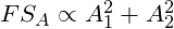
This would result in a reduced combat effectiveness. For example, a force 50 strong would have a strength proportional to 502 (or 2500). The same force divided into two groups of 25 would have an effectiveness proportional to 252 + 252, or merely 1250; one half, in fact, of its value as a cohesive unit.

We will now look at an application of this principle to the study of naval history, as found in Lanchester’s original work.

CONCENTRATION AND THE LINE OF BATTLE

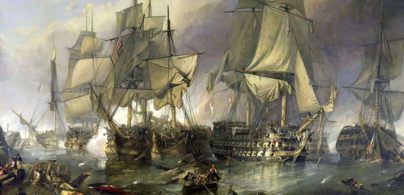
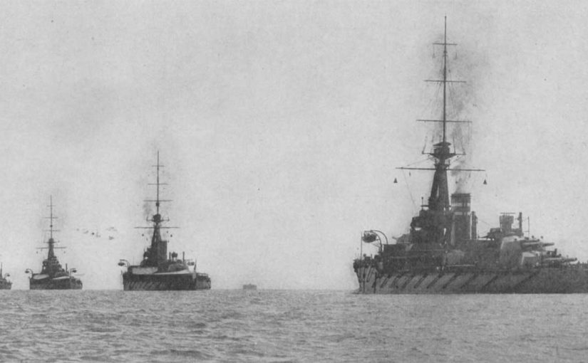
From the mid 17th century, about a hundred years into what has come to be known as the Age of Sail, it became standard practice for fighting navies to do battle in a line formation. This seems a natural development, as ships were generally designed to fire abeam; the line ensured that no ship masked the guns of another.

The French line firing upon the British columns at the Nile, 1798
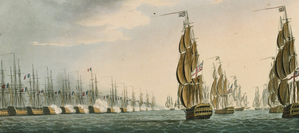
(painting by Thomas Whitcombe)

Perhaps more importantly, in an era before the invention of wireless telegraphy, and with ship formation lengths often exceeding the nautical mile, the line was relatively easy to keep and manoeuvre, and could be led somewhat effectively from its middle; when in doubt, all a captain had to do was follow the ship ahead.

However, the limited traverse and range of naval guns in this period made it unlikely that two consecutive ships in the formation would be able to overlap their fire – and virtually impossible that three would do so. As a means of concentrating firepower, therefore, it was not the most efficient. Wayne P. Hughes Jr. tells us:

It is proper therefore to think of the column itself primarily as a means of controlling the force inherent in the admiral’s ships and only secondarily as a means of effecting concentration of firepower.

Hughes Jr, Wayne P. – Fleet Tactics and Coastal Combat (1999)

Under such restrictive tactical conditions, naval engagements (especially those between fleets of comparable sizes) would often prove indecisive, with neither side exerting true concentration of force. As Charles Henri d’Estaing would put it, naval battles often produced “more noise than profit”.

Historical literature frequently describes as ‘decisive’ those actions in which the conventional line was abandoned: Lanchester and Hughes refer to the Battle of the Saintes of 1782 (known to the French authors as the Battle of Dominica) in which Sir George Rodney defeated the Comte de Grasse by breaking the French line at three places, enveloping the resulting segments, and engaging them in detail. Similar dispositions were employed successfully by John Jervis at Cape St. Vincent, and Adam Duncan at Camperdown, in 1797. A year later, Lord Nelson carried the day at the Nile by separating his fleet into divisions, and doubling on the French van.

We could be tempted to believe that adopting these modern tactics was in every case desirable, and blame all who did not for a lack of awareness of what seemed to be a clear trend. But we must bear in mind that, in breaking the formation, concentration of fire was obtained at the expense of the ability to actively lead the fleet; the line of battle was, above all, an instrument of command and control, and without it there was little chance of issuing new orders or adapting to emerging situations. Anything that had not been carefully planned and drilled beforehand would be left, once the first shot was fired, to the discretion and best judgement of each captain. It was a gambit that not every navy could afford.

THE BATTLE OF TRAFALGAR

In his memorandum to the combined fleet at Toulon before Trafalgar, French admiral Pierre-Charles Villeneuve echoes this tactical outlook:

The enemy will not content himself with merely forming a line of battle parallel to ours, and so engaging us in an artillery combat wherein success falls often to the side that is more skilful, but always to the side that is more lucky. He will try to surround our Rear, to cut through us, and to bring to bear groups of his own ships upon those of ours that he has isolated in order to envelop and crush them.

James, William – Naval History of Great Britain, vol. III (1837)

His description of how the battle would play out is remarkably accurate, and reproduces Horatio Nelson’s own original plan almost to the letter. This tells us two things: first, the British strategy was really no surprise to anybody – we have mentioned already many precedents from which lessons had been duly learned. Second, there was not much Villeneuve could do about it, even if he knew in advance. A fleet had to be drilled and coordinated to a remarkably high standard in order to operate outside the constraints of the traditional line of battle, and the French admiral had no means of parrying the blow.

MODELLING THE BATTLE

Furthermore, the British could hardly have expected a clear victory by keeping the line. Nelson himself, in his 1805 memorandum, argues it would have been:

[…] almost impossible to bring a Fleet of forty Sail of the Line into a line of battle in variable winds, thick weather, and other circumstances which must occur, without such a loss of time that the opportunity would probably be lost of bringing the enemy to battle in such a manner as to make the business decisive.”

James, William – Naval History of Great Britain, vol. III (1837)

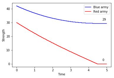
To the difficulties of manoeuvre we must add a discouraging numerical disadvantage, which would have been most apparent in a prolonged cannonade at long range. In Aircraft in Warfare, Lanchester uses his Square Law to predict the likely outcome had the old tactics been adhered to. The analysis begins with the hypothetical scenario of 40 British sail of the line facing 46 from the Combined Fleet, as originally predicted by Nelson.

Direct confrontation between the forces expected by Nelson

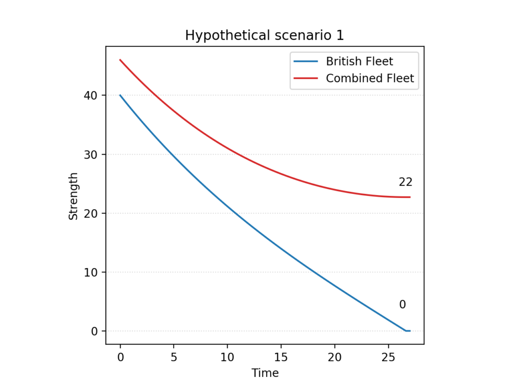
The Franco-Spanish fleet would be expected to win, and by a wide margin, assuming the ships and crews on both sides to be equal. Just to achieve parity, the British fleet would have needed a qualitative advantage of roughly 32 percent.

If we look instead at the numbers ultimately engaged in the battle, the British disadvantage is even more dire. In the proceeding of the 20th International Conference on Technology in Collegiate Mathematics (ICTCM) of 2009, William P. Fox of the Naval Postgraduate School does the same calculation as Lanchester, but for the historical 27 sail of the line under Nelson facing Villeneuve and Gravina’s 33:

Direct confrontation between the forces actually engaged

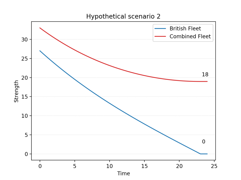
In this case, the model predicts that the British ships would have to fight almost fifty percent more efficiently to compete on equal terms.

It is worth noting that, as represented here, both scenarios show the opposing fleets just holding alongside at some distance, and pounding away at each other until the utter destruction of either, or both. No analyst would even begin to believe that, of course: the purpose of Lanchester’s equations in situations such as these is merely to estimate the relative advantage of one side over the other, not the final result of an engagement. In the absence of an obvious edge of manoeuvre that would prevent the enemy from withdrawing, a more likely outcome would be an indecisive exchange of fire after which, in the poignant words of the comte d’Estaing, the sea would “remain no less salty than before”.

THE SUM OF ITS PARTS

We know Nelson did not lose – and as Fox tells us, without a clear numeric or qualitative advantage over the Combined Fleet, the only option would have been a change in strategy.

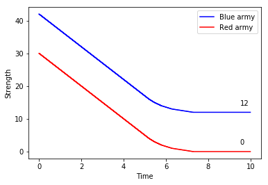
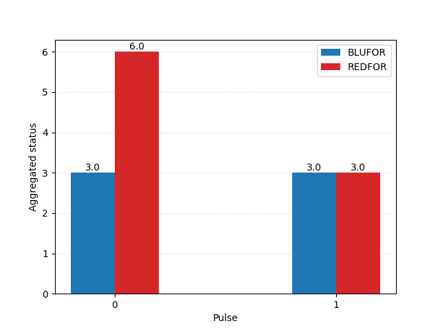
A simple but elegant explanation can be found in Lanchester’s original work, as he analyses the rough sketch of a battle plan found in Nelson’s original memorandum of 1805. The Square Law, we remember, tells us that the fighting power of a formation is proportional to the square of its numerical strength. Prior to the battle, the British admiral expected to be able to bring 40 sail of the line into the action, to the enemy’s 46. Looking at the numbers behind one of the charts we saw earlier, we note that each side’s relative strengths would be:

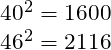
Assuming no qualitative upper hand to either side, the British fleet would be at a disadvantage of 516 – or roughly 32%.

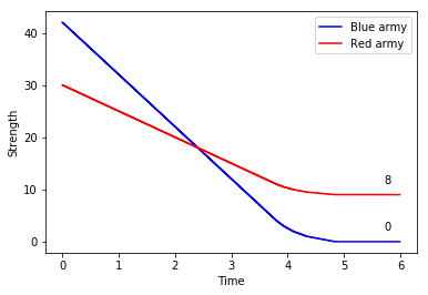
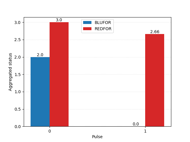
Rather than face these unfavourable odds in a direct clash, Nelson’s plan was to split the Franco-Spanish line into two. To achieve this, he would detach his eight fastest two-deckers to engage and occupy the enemy’s van, while the isolated rear was overwhelmed by the remaining 32 British ships. The analysis must now gauge the relative strengths of these smaller groups separately:

Which would give the British an advantage of 30 – just shy of 3% – over the Combined Fleet.

THE SQUARE LAW WITH REINFORCEMENTS

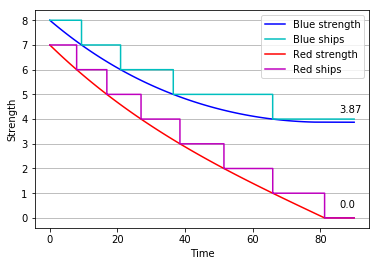
Alternatively, we could model the battle as a series of smaller, consecutive actions, in which different parts of each fleet join the fray at different times. This is not unreasonable, since Nelson’s plan was precisely to use his weather column (led by his own command HMS Victory) to isolate the van of the Combined Fleet, and keep it from supporting the rest of the formation in the first stage of the action.

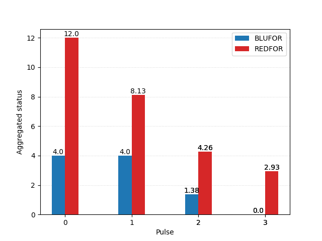
That is the approach chosen by W.P. Fox in the proceeding of the 20th ICTCM. In his model, Nelson’s fleet of 27 sail of the line is divided into two columns, sized 13 and 14. They sail through the Allied formation in two places, separating it into three groups of 17 (rear), 3 (centre), and 13 (van).

J.G. Bartholomew, – A Literary & Historical Atlas of Europe (New York, 1910)

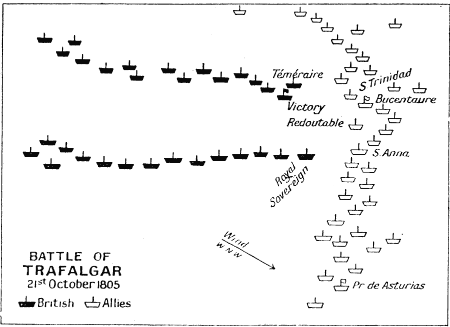
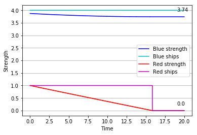
The British column of 13 first engages the enemy’s three centre ships, quickly overpowering them. They are then joined by the 14 ships in the reserve, and together they tackle the more numerous enemy rear. There, too, they gain the upper hand, and finally direct their attention to the last 13 sail in the Franco-Spanish van.

The Battle of Trafalgar as three consecutive actions

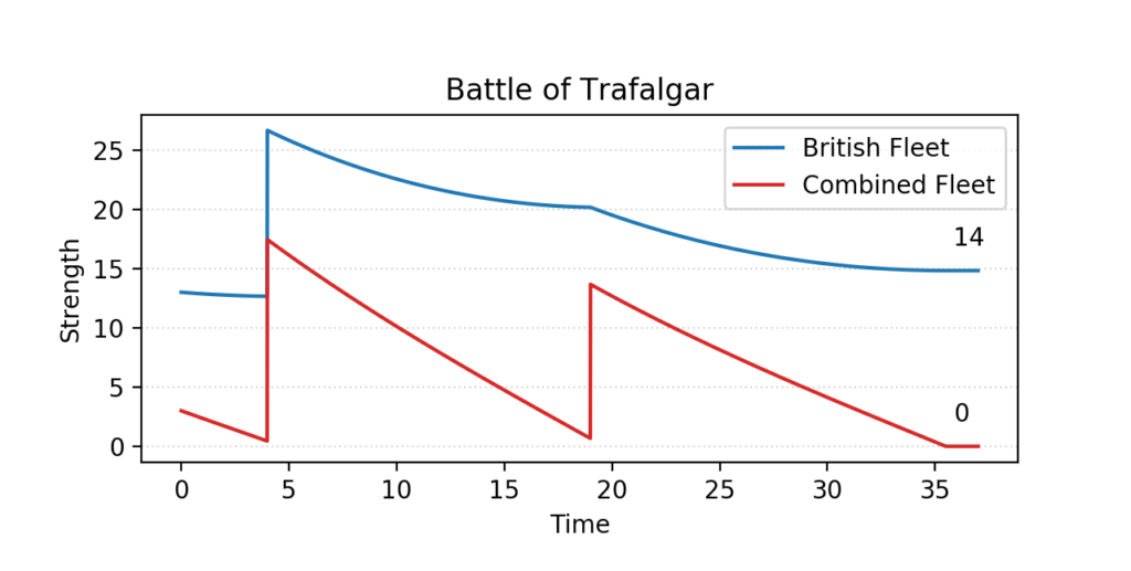
In this scenario, the British fleet not only seizes victory, but even does so with a comfortable margin – its remaining forces are equivalent to the combat power of 13 to 14 intact ships, which is about one half of its original strength; the Combined Fleet, in spite of having a slight numerical advantage at first, is completely annihilated.

READING INTO THE RESULTS

Fox’s model represents the battle in three distinct phases, which take place in order. This might give us the illusion that it is a high resolution model – meaning, it tells us in some detail what is happening when. It is important to remember that it is not, and in fact no application of Lanchester’s square law ever had that pretence.

What it does clearly expose is that numbers (of ships, of men, of guns) mean little without a context. A battle is a complex event, formed organically by numerous smaller clashes; numerical superiority, of course, is a clear advantage in any one of them. But it is within the domain of tactics to ensure that we have this advantage where and when it can lead us to a favourable result. Nelson could not have won without concentrating his forces intelligently; the judicious application of the same principle had granted him victory before, as it had Jervis, Rodney, and Duncan. As its author originally intended, the Square Law remains today an eloquent demonstration of the merits of force concentration.

GitHub

The Python implementations of the models used in this article for plotting simulated combat results can be found in the author’s GitHub page.

FURTHER READING

Share this article:

Hughes’ Salvo Model

Share this article:

Many attrition models represent armed combat as two uninterrupted streams of fire between the opposing sides – that is, both forces are assumed to be causing and suffering casualties every instant of the engagement.

This allows the analyst to study casualty rates over arbitrarily small increments of time. We refer to these models as continuous or differential models (for their use of differential equations) and the original formulations by Lanchester and Chase, as most of their later revisions by other authors, belong in this category.

Of course, no real exchange of fire is truly “continuous” in the strict sense. One can reasonably expect pauses and changes of pace to exist, and there is no such thing as a fractional bullet or shell to begin with. In this apparent shortcoming, differential combat models showcase an important characteristic of mathematical models in general: the focus is placed on relevance, rather than on realism. We know that discontinuity may exist, but we choose to neglect it when we know that it will not affect our analysis in any significant way.

This assumption can be reasonable in some scenarios, such as prolonged fighting over many days (Engel’s analysis of Iwo Jima, or MacKay’s for the Battle of Britain) or engagements in which large volumes of fire are exchanged with relatively little pause (Lanchester’s own study of the Battle of Trafalgar). In these conditions, even if modelling does not always manage to yield a reasonable fit to reality, it can at least provide some valuable insight on the relationships between the input parameters – and sometimes that is plenty enough. In the words of Clausewitz:

“If theory investigates the subjects which constitute war; if it separates more distinctly that which at first sight seems amalgamated; if it explains fully the properties of the means; if it shows their probable effects; if it makes evident the nature of objects; if it brings to bear all over the field of war the light of essentially critical investigation,—then it has fulfilled the chief duties of its province.”

DISCRETE EVENTS

There are some scenarios, however, in which discontinuity is far from irrelevant.

Advances in military technology throughout the 20th century, particularly in the realm of naval warfare, allow combatants to deliver great amounts of firepower in very short time frames. Torpedo spreads, carrier strikes, and missile salvos deal damage suddenly and violently, often deciding the outcome of a battle in one or two swift blows – a ship might be fully operational one instant, and out of action the next.

This increased punctual lethality of weapon systems, combined with greater ranges of engagement, have turned naval warfare into a mostly discrete (rather than continuous) reality: whatever the duration of a battle might be, the actual exchange of fire is reduced to a few short and clearly separated instances in which vast amounts of damage are dealt. An immediate implication is that one side may surprise the enemy, hitting them before they are able to react – in contrast to gunnery duels, in which unanswered fire is rare.

In these circumstances, time-continuous modelling simply does not cut it, as its theoretical framework is too far removed from the nature of reality. A new approach is necessary.

THE SALVO MODEL

In his 1986 classic Fleet Tactics: Theory and Practice, USN captain Wayne P. Hughes Jr. explores the nature of pulsed combat, beginning with a simple mental exercise on the nature of carrier actions in the Second World War. Hughes begins with the reasonable assumption (somewhat justified by historical data) that one carrier air wing or CVW (known as “Carrier Air Groups” until 1963) could sink or cripple, on average, one enemy carrier in a single sortie.

In what he refers to as a “very rudimentary table”, Hughes shows the expected outcomes of a surprise strike of a force B on a force A, after which any survivors from A are allowed to counterattack:

Initial Force (A/B)2/24/33/22/13/1
Survivors (A/B)0/21/21/11/02/0

In the next few pages of the chapter, this simple rule of thumb is applied to a series of carrier battles of 1942 (The Coral Sea, Midway, Eastern Solomons, Santa Cruz Islands, and the Philippine Sea) obtaining a surprisingly good fit. Later on, the model is slightly altered to account for the effect of defending fighters, which would reduce the striking power of attacking bombers by shooting down or disrupting their formations. In essence:

\textrm{Carriers out of action} = \textrm{Air wings launched - Fraction defeated by fighters}

This elementary theoretical tool serves as the foundation for a model of modern combat between missile-equipped warships – very similar in many aspects to carrier actions. In such scenarios, anti-ship cruise missiles (ASCMs) take the place of bomber formations, and point defence systems and SAM batteries fill in for defending fighter patrols, but the process remains much the same:

  • The attacking side launches a number of missiles at detected enemy elements from beyond visual range.
  • The defender attempts to intercept or distract as many of the incoming ASCMs as possible.
  • A fraction of the missiles overwhelm the defences or otherwise leak through them, and hit their intended targets, which suffer damage until a threshold is reached and they are rendered out of action.

In a later paper in 1995, titled A salvo model of warships in missile combat used to evaluate their staying power, Hughes constructs the analytical skeleton for this model as follows:

ASSUMPTIONS

Two sides (let us call them Blue and Red) are each made up of identical missile-armed warships. We use the letter A to represent the force strength (in number of warships) of the Blue side, and B for that of the Red side.

Each individual warship has a fighting or striking power, reflecting how many well-aimed missiles it can fire in one salvo. This is α for Blue ships, and β for Red ships.

Warships also have a defensive power, being the number of missiles they can shoot down from an incoming barrage. For consistency with Hughes’ work, we will call this a3 for each ship in the Blue side, and b3 for the Red side.

Finally, warships are also defined by their staying power (a concept previously explored by J.V. Chase in his classified paper of 1902) being the number of hits they can take before being rendered out of action. This we call a1 for Blue ships, and b1 for Red ships.

This established, the process of an attack by A on force B would go like this:

  1. All ships of force A fire at the enemy, with all their good shots grouped into one large salvo.
  2. All ships of force B collectively fire their defensive SAMs at the incoming salvo, shooting down some of the incoming missiles.
  3. The remaining missiles hit force B and distribute their damage uniformly among all available targets.
  4. It is important to note that both striking and defensive firepower are, in Hughes’ original formulation, dependent on a ship’s status: an undamaged ship will always enjoy its nominal values, but as it suffers hits, its offensive and defensive capabilities will be proportionally reduced.

Depending on the scenario we wish to explore, A and B can attack each other simultaneously, or one can surprise the other. Either situation can happen an arbitrary number of times or until one side is wiped out.

BASIC EQUATIONS

The mathematical equations describing this process are known as the Basic Salvo Equations:

\Delta A = \frac{\beta B - a_{3}A}{a_{1}}

\Delta B = \frac{\alpha A - b_{3}B}{b_{1}}

An example engagement using this basic formulation is offered in McGunnigle (1999) Appendix A, p.71, with the following input data:

BlueRed
Units36
Striking pwr.31
Defensive pwr.21
Staying pwr.21

And these results plotted per time pulse (salvo):

In this example case, the Blue side can fire nine missiles (three per ship) and intercept six, whereas Red can fire six missiles (one per ship) and intercept another six. Blue, then, can intercept all of Red’s ASCMs and survives the salvo unharmed. Red is predictably not so fortunate, as three of Blue’s missiles overwhelm its defences and knock three ships out.

EMBELLISHED MODEL

The model is further developed by many authors, the first being Hughes himself, to account for other possible factors. The additions are often in the form of fractional coefficients (values from 0 to 1) reducing the original parameters to reflect various realities of naval combat. Some examples would be:

  1. Scouting – affecting total striking power, and representing the fraction of the enemy that a side can actually engage based on sensor range or precision, off-board scouting assets, etc. For instance, a side with a scouting coefficient of ‘0.5’ would only be able to engage one half of the enemy fleet successfully, so its striking power would be reduced by 50%.
  2. Defensive alertness – like scouting, but affecting defensive firepower instead. Used to reflect how prepared a group is to successfully fend off an attack.
  3. Training – affecting both striking and defensive power.
  4. Weapon reliability and accuracy – affecting the probability that shots (offensive or defensive) will hit, to reflect imperfect guidance or firing solutions, manufacturing flaws, etc.

Jeffrey R. Cares provides a variety of scenarios between Knox-class frigates using this kind of embellished model, and data gathered from NAVTAG exercises, in his 1990 paper The fundamentals of salvo warfare. Here is one such encounter taken from page 23 (Scen. VI):

BlueRed
Units23
Striking pwr.44
Defensive pwr.44
Staying pwr.22
Scouting11

Cruise missiles in the model are assigned an accuracy of 0.61 (roughly three fifths are expected to hit) while defences are given an effectiveness of 0.35. These numbers are obtained from the results of the NAVTAG simulation.

The engagement, plotted in our own Python implementation:

This scenario showcases the importance of concentration of force, in a way that is somewhat reminiscent of  Lanchester’s Square Law: with a local numerical superiority of one ship (50% advantage) REDFOR manages to disable all of BLUFOR’s ships, losing none of their own.

Other revisions to the model have been proposed, such as reworking defensive firepower calculations to account for ‘leakers’ – the (hopefully for the defender) small fraction of missiles that are expected to always bypass protective systems , due to the practically limited reliability of chaff and flares, point defence weapons, etc. Yao Ming Tiah (2007) provides a thorough evaluation of scenarios following this rule, of which we detail one (excursion A3, pp. 26 – 29):

BlueRed
Units412
Striking pwr.84
Defensive pwr.62
Staying pwr.1.51
Scouting0.60.6

Tiah assigns missiles a launch reliability of 0.9 (one in ten fails to launch) and an accuracy of 0.7. Defences have an aggregated effectiveness of 0.68. Blufor surpises Redfor and attacks first.

Here is the corresponding plot obtained from our implementation:

Though ultimately losing the engagement, the heavily outnumbered BLUFOR manage to put just under four of REDFOR’s ships out of action in their surprise attack – almost enough to level the playing field.

STOCHASTIC MODEL AND SIMULATION

All variants of the Salvo model included here are deterministic: given the same input data, they will always produce the same output. As is the case with all deterministic models of combat, the result is meant to be the average expected outcome, not an infallible prediction. War is a chaotic affair by nature, and the purpose of modelling is finding out what can reasonably be expected, rather than a monolithic truth.

However, we might also be interested in the variance (how much can we expect reality to differ from our prediction?) and the distribution (what is the relative probability of a given outcome?) of the possible results.

In this spirit, Armstrong (2004) develops a stochastic version of Hughes’ model, in which some of the parameters are introduced as mean values with a known variance, rather than being fixed. He and Powell use this approach in a 2005 paper to model possible outcomes of the Battle of the Coral Sea.

Another option (used earlier by McGunnigle and Lucas in 2003) is simulation: one or more events (say, a missile hitting its target, or an enemy ship being detected by sensors) are assigned a probability, be it from past combat experience, weapon specifications, or data gathered from tactical exercises. This done, we resolve one instance of the engagement, determining whether these events do happen by using a random process of our choice – today we would use a pseudo-random number generator on a computer, but suffice it to say we are doing a sophisticated roll of the dice, as if we were playing a board game. We then repeat the operation a few thousand times, recording the results for each instance. All that is left is mapping how many times each of the possible outcomes have occurred.

Whichever approach we choose, the result will be similar: instead of an estimated mean prediction (as with the deterministic model) we will obtain a probability distribution of the possible outcomes, which might prove much more valuable for our analysis – especially if our objective is assessing risk.

An additional perk of the stochastic variant is that the need to apply damage uniformly is lifted: missiles can be assigned randomly or semi-randomly to targets using whatever distribution best fits our purposes. As a notable example, Kevin G. Haug published a paper in 2004 in which he experimented with the application of a Pólya urn distribution to missile targeting in the salvo model.

CONCLUSIONS

Elegant and powerful in its simplicity, the salvo model offers a solid foundation for understanding the relationships between various factors in modern naval combat. Hughes himself highlights a few of his own conclusions in the original 1995 paper:

  • Superiority in numbers provides a reliable advantage on its own: if side A’s ships have twice the striking power, defensive power, and staying power as side B’s, B can still achieve parity by having twice as many ships as A. Refer to the scenario shown from Cares (1990) earlier in this article.
  • Of all parameters taken into account, staying power (the ability of a ship to sustain damage) is the only one that is unaffected by poor tactical choices.
  • As J.V. Chase pointed out, staying power does not scale linearly with ship displacement: a ship twice as large is not necessarily twice as hardy. Striking and defensive power can be increased more easily and cheaply, which leads to modern fleets having large destructive potential relative to their ability to sustain damage.
  • This causes ‘tactical instability’: small changes in the engagement can lead to grossly different outcomes. A single missile hitting or missing might mark the difference between victory and defeat, as that is often enough to cripple one target entirely.
  • In such unstable situations, scouting – the ability to detect the enemy and strike first – becomes paramount. Even a superior fleet must strive whenever possible to land the first blow, as a single salvo from a comparatively inferior opponent is potentially disastrous. The scenario taken from Yao Ming Tiah’s (2007)  illustrates this principle.

GitHub

The Python implementations of the models used in this article for plotting simulated combat results can be found in the author’s GitHub page.

FURTHER READING
  1. Hughes, Wayne P., Jr. – A Salvo Model of Warships in Missile Combat Used to Evaluate Their Staying Power (1995)
  2. Cares, J.R. – The Fundamentals of Salvo Warfare (1990)
  3. McGunnigle, John – An exploratory analysis of the military value of information and force (1999)
  4. Armstrong, Michael J – A stochastic salvo model for naval surface combat (2004)
  5. Haugh, Kevin G. – Using Hughes’ Salvo model to examine ship characteristics in surface warfare (2004)
  6. Tiah, Yao Ming – An analysis of small navy tactics using a modified Hughes’ salvo model (2007)
Share this article:

Attrition Models at Sea

Share this article:

The Lanchester Square Law of 1914 is, by design, limited in scope. The author did not concern himself with victory or defeat, advance or retreat, or control over a given area of land; attrition rate (casualties inflicted and suffered over time by the contending sides) is its only output, and any deeper insights are left to the practitioner’s best judgement.

Some have questioned its validity for exactly this reason, arguing that combat is much more complex than a mere exchange of fire and an ensuing butcher’s bill. And it is a valid point; but as James G. Taylor reminds us, we should not be too ready to blame a model for our incorrect implementation of it, or for not validating satisfactorily in a scenario it was never designed to describe. In its original form, Lanchester’s Square Law is an attrition model and nothing else.

This could help explain why the first proposals of a similar set of equations were originally offered by Navy men – J.V. Chase, Bradley A. Fiske, and Ambroise Baudry. At sea, there is a predominance of attrition over manoeuvre: as Wayne P. Hughes points out in his classic reference work Fleet Tactics and Coastal Combat, “Forces at sea are not broken by encirclement; they are broken by destruction”. An attrition model may never take us beyond a mere casualty count in a land battle, but in the realm of naval action it might be just good enough.

There are other factors that make the sea an ideal testing environment for the practitioner of Operational Research. Hughes continues:

“The potential to effect this concentration [of force] is greater at sea than on land. At sea there is no high ground, no river barrier, no concealment in forests that requires what is often used as a rule of thumb on land, a 3:1 preponderance of force to attack a prepared position […]. Sun, wind, and sea state all affect naval tactics, but not to the extent that terrain affects ground combat.”

He concludes that the main objective of naval tactics throughout history has been the successful attack, and that is achieved by concentration of firepower – Lanchester would have agreed. Although today we still refer to the Square Law as Lanchester’s creation and by his name, it can be argued that the models created by Chase, Fiske and Baudry not only predate it, but are also more fortunate in their application from their conception, being better adjusted to the reality of war at sea.

THE MODEL

As presented in 1902, Lieutenant J.V. Chase’s own approach to the Square Law made the following assumptions, very similar to what Lanchester would postulate a decade later:

  • When averaged out, shell fire from a fleet can be considered a continuous stream, rather than a series of individual projectiles.
  • The two opposing fleets (let us call them Blue and Red) participating in the action are homogeneous: all ships in the Blue fleet are identical, and so are all ships in the Red fleet.
  • The fighting power of a given ship is constant: it is unaffected by range, target aspect, spotting effectiveness, or morale.
  • All ships in the fleet are able to fire at all ships in the opposing fleet, and no shots are wasted on a target that is already out of action.

The variables that describe the encounter are:

  • The fleets engaged each have a number of ships, which we will refer to as A and B respectively.
  • Ships have a “fighting power”, which we define as the number of accurate shots each of them can fire in a given unit of time. All ships in a fleet are assumed to have the same fighting power. We refer to the fighting power of Blue’s ships as α, and that of Red’s ships as β.

Finally, and as the main deviation from Lanchester’s formulation,

  • Ships are also defined by their “staying power”: the number of shots they can withstand before being taken out of action. Again, all ships in a fleet are expected to be identical in this regard. We write the staying power of Blue’s ships as a, and that of Red’s as b.

It is worth mentioning that ships are, in this model, not necessarily taken out of action one by one: one intact ship is equal in every way to two ships that are halfway out of action. For this, we will refer to the results of Chase’s equations as the “equivalent” number of surviving ships, which represents the remaining combined combat strength of the fleet rather than an exact number of vessels.

The mathematical formulation, as presented by Wayne P. Hughes in The value of warship attributes in missile combat (1992) would look like this:

\frac{dB(t)}{dt} = \frac{\alpha A(t)}{b}

\frac{dA(t)}{dt} = \frac{\beta B(t)}{a}

Where A and B are the number of ships in the Blue and Red fleets, α and β their fighting power, and a and b their staying power.

The state equations for a given time, obtained by integration:

\alpha a[A(0)^{2} - A(t)^{2}] = \beta b[B(0)^{2} - B(t)^{2}]

A “square law” much in the spirit of Lanchester’s, and an identical attrition process being described. The only new factor, from a mathematical perspective, is the notion of “staying power”.

This difference might seem small at first (a mere denominator) but it is invaluable in practice: the model lets the practitioner explore the relative values of offence and defence, which in this formulation affect the end result equally, all else being the same. Chase himself, in a 1921 retrospective on his work, reflected:

“Having certain definite quantities of the various materials the question of ship design [is], …in the simplest form: “Shall we construct from these materials one ship or two ships?”…if we decide to build one ship instead of two, this single ship must be twice as strong offensively and twice as strong defensively as one of the two ships.”

History has taught us that fighting ships are susceptible to catastrophic damage; a torpedo strike, a bomb exploding below decks, or even a really unfortunate shell hit can take a well-armoured vessel out of action. This should make it abundantly clear that a ship twice the displacement of another is not necessarily twice as strong defensively. A design trend towards smaller vessels would seem mathematically reasonable.

As for the value of the concentration of firepower, let us run the experiment Chase proposed in the same retrospective we mentioned earlier.

A PRACTICAL CASE

Say we have two opposing fleets, both identical in every aspect.

Each has eight ships of comparable power; for the sake of our example, let us say all of them can fire on average 0.2 accurate shots per time increment, and all of them can take, say, twelve shots before they are disabled.

Of course, two such fleets (with identical combat strength and staying power) would eventually annihilate each other if they attacked at the same time and neither retreated.

Instead, let fleet Blue manoeuvre in such a way that one ship of fleet Red is masked and unable to fire. The contest is now temporarily eight ships versus seven – an apparently small imbalance. We apply the equations and plot the strength of both fleets as a function of time:

Phase 1 plot

Predictably, the larger fleet wins this first phase of the engagement. We might find it more surprising that it does so by a comfortable margin, with the equivalent of 3.87 ships still in the fight – almost one half of the fleet’s original strength. These could now engage the lone remaining hostile ship, as shown below:

Phase 2 plot

The last ship of fleet Red is eliminated with minimum damage to Blue – now at the equivalent of 3.74 battle-ready ships.

And so, a minor alteration in the initial conditions of the action grants fleet Blue a decisive victory, preserving almost half of its original force.

LESSONS

Chase’s model is a testament to the importance of concentration: the side engaging the fewest enemies while bringing the most guns to bear can expect to win, and manoeuvre should aim to secure this advantage. This much should be evident from our earlier example.

It also makes a compelling argument for the desirability of smaller ships. With offensive power and staying power having equal weight, the latter simply cannot be relied upon; the effects of enemy fire are difficult to quantify, and the possibility of catastrophic damage poses a great risk to any fleet concentrating its resources.

However, and perhaps more importantly, it shows how the shortcomings of attrition models are less conspicuous in the setting of naval warfare than they are on land; context matters.

GitHub

The Python implementations of the models used in this article for plotting simulated combat results can be found in the author’s GitHub page.

Further reading

  1. Wayne P. Hughes – Fleet Tactics and Coastal Combat
  2. Wayne P. Hughes –  The Value of Warship Attributes in Missile Combat
  3. James G. Taylor – Lanchester-type Models of Warfare, Vol. I
Share this article:

Lanchester’s Laws of Combat

Share this article:
Early combat models

Just over a hundred years ago now, US Navy lieutenant (later rear admiral) J.V. Chase developed a differential equation to model engagements between two homogeneous fleets. About a decade later, British engineer Frederick W. Lanchester arrived independently to an almost identical equation, with examples covering air and land combat as well. A Russian contemporary to both, M. Osipov, also reached similar conclusions in a paper published in the tsarist journal “Military Digest” (Voennyi Sbornik) in 1915.

Of the three, history has been kinder to Lanchester: Chase’s work was not declassified until 1972, too late for him to enjoy the public recognition he rightly deserved; and Osipov, although sometimes mentioned alongside his British counterpart, is still a relative stranger to us.

In practical applications, the simple combat models described by Lanchester and his contemporaries are mostly surpassed today – partly because of the more complex and dynamic nature of the modern battlefield, but mostly due to the power of calculation brought by the computer age, which makes much more sophisticated simulations possible.

And yet, Lanchester’s Laws, as we know them today, never quite seem to lose relevance. Many combat models introduced in the last few decades are directly evolved from them (COMAN, Bonder-Farrell), or use them at the local level to describe smaller engagements within a broader framework.

Lanchester’s Linear Law

Lanchester began by postulating a simple yet reasonable condition of ancient combat (close formations of men using swords or spears) in what he called the “Linear Law”: a combatant armed with a melee weapon can only engage one target at a time, within arm’s reach. What this means is that the casualties that a force could sustain or cause at any given instant have a practical upper limit, proportional to the number of its combatants that are in direct physical contact with the enemy. At most, this upper limit would be the number of active units in the smaller force, but further limitations could be imposed by terrain, or formation frontage. We will now examine an example of the latter:

In the situation above, and given equal fighting skill for both sides, the Blue army and the Red army would cause the same exact number of casualties (five) per unit of time and would go on like that until the smaller army (in this case, Red) were wiped out.

From the Blue army, 12 units survive the encounter.

Now, let us imagine the Red army is technically superior to the Blue army: due to a greater fighting skill, or better equipment, or a combination of both, any Red soldier can eliminate two enemies in the time it takes a Blue soldier to eliminate just one. In that case, the plot of the forces of both sides as a function of time would look like this:

Red wins this time around, with eight survivors.

We can make the following observations from these two engagements:

  • The attrition rate of both armies is constant throughout the battle (except by the end, when fewer soldiers remained than would fit the original frontage)
  • A larger army does not confer a greater killing power – only a greater staying power, as the larger army can soak up more casualties before being eliminated.
  • An army that is outnumbered two to one can compensate by being exactly twice as lethal. In other words, lethality and numbers have the same weight in deciding the outcome of a battle.
  • Frontage does not really alter the outcome of the battle, only its duration.

According to Lanchester, exactly the same rules could be applied to a modern scenario of unaimed fire, in which both sides fired at an enemy they could not see, and merely swept a constant target area: in such a case, the larger side would have greater firepower, but this would be compensated by a lower density of enemy targets; the outnumbered side would have fewer guns, but their shots would find their mark more often. The result would be a constant attrition rate for both armies, exactly as in the melee combat examples above.

Lanchester’s Square Law

In modern combat using long range weapons and aimed fire, Lanchester continued, the restriction established by the Linear Law is lifted: now, any combatant can engage any target in range, and in turn receive fire from multiple enemies. Thus, attrition rate is no longer limited by frontage – every element can participate in every stage of the battle.

In these conditions, if an army had 20 fighting elements, and each were expected to eliminate one enemy unit on average every two “time steps” of a given encounter (whatever we actually mean by a “time step”, be it a minute or a day, depends on the scope of our simulation) then the army would be expected to eliminate 10 enemies on average per time step. In a general case, an army with a number of elements A, all of which participate in the encounter in one time step, will always cause a number of casualties to an army B of A times α, where α is the expected number of kills per element per unit of time on average. This translates into the following equations:

\frac{dB}{dt} = -\alpha A

\frac{dA}{dt} = -\beta B

Where A and B are the number of soldiers in each army, and α and ß their average expected number of kills per soldier per unit of time. Today, we refer to α and ß as Lanchester attrition-rate coefficients.

Let us apply these equations to our prior example of a Blue army numbering 42 soldiers, and a Red army with a strength of 30. As before, we make both armies exactly as lethal – both will be expected, for this example, to neutralise one enemy every five time steps (1/5 = 0.2 kills per time step). Substituting these values in the previous equations, we obtain:

\frac{dA}{dt} = -0.2 \times 42

\frac{dB}{dt} = -0.2 \times 30

Which, plotted as a function of time, gives the following result:

In our Linear Law example, with the same numbers, the Blue army won with only 12 surviving units. This time around, applying the Square Law, things are considerably more lopsided, as 29 elements of Blue survive unscathed.

Intuitively we can appreciate how, in the conditions established by Lanchester’s Square Law, superiority in numbers has a greater effect in the outcome of an encounter than the lethality of each individual unit – every casualty inflicted not only reduces the number of enemies that can fire back, but also increases the concentration of fire on each target in the next time pulse. A tacit agreement with Nathan Bedford Forrest’s military maxim “get there first with the most men”.

Analytically, we may divide the equations for the casualty rates, obtaining:

\frac{dA}{dB} = \frac{\beta B}{\alpha A}

Which we can rewrite as:

\alpha A \times dA = \beta B \times dB

to relate the instantaneous losses of both armies, and then integrate to find that:

\alpha(A_0^2 - A^2) = \beta(B_0^2 - B^2)

Which shows that the fighting strength of an army is proportional to the square of its size – hence “Square Law”.

Validation of Lanchester’s Square Law:

As a combat model, Lanchester’s Square Law has some considerable limitations, among others:

  • It assumes perfect intelligence, as both sides know the exact location of the enemy at all times.
  • It assumes perfect fire control, as both sides can concentrate fire in the most efficient way.
  • It assumes the conditions of the battlefield are constant, as the efficiency coefficients α and ß are unaffected by changes in terrain, manoeuvres, morale, supply, etc.
  • It is a deterministic model, as the same input will always yield the same result.
  • It is a homogeneous model, in that all elements of a combat unit are assumed to have the same fighting characteristics.

Many authors have proposed revisions and expansions of Lanchester’s work to correct some of these shortcomings, or to account for a variety of factors such as reinforcement and withdrawals, operational losses, command and control, guerrilla warfare and insurgency, the suppressive effects of weapons, close air support, etc. A detailed list of these developments up to the late 1970s can be found in James G. Taylor’s Lanchester-Type Models of Warfare, vol. I, 1980.

This said, we must look at the Square Law not as a combat model, but as an attrition model. In other words, we cannot expect it to paint a detailed view of the evolving battlefield, but rather to describe the mathematical process by which casualties are dealt and sustained, once all other factors are known.

And in that regard, it can do surprisingly well. Although other studies exist that illustrate the matter clearly, J.H. Engel’s 1954 paper on the battle of Iwo Jima shows a remarkable fit between theoretical vs. actual attrition rates using Lanchester’s Square Law:

Conclusions

On the subject of Lanchester models of warfare, Professor James G. Taylor said in 1980:

We should, perhaps, be more amazed that such simple models yield intuitively appealing results than be critical because of the factors omitted from them. As is usually the case with simple analytical models, they may be too abstract to solve any specific real operational problem. They can, however, illustrate a general principle such as concentration, clearly delineate modelling issues, warn about potential difficulties, and serve as a basis for communication among analysts

Whether Lanchester models continue being practical is a different debate entirely, but one cannot deny that they continue being relevant, both in the field of Operational Research and outside it. The civilian study of military history, in particular, strikes us as a doctrine with no need to solve specific operational problems, but which could do with some insights into the dynamics of combat – a historian would not do far too wrong revisiting some past conflicts from an analytical perspective.

GitHub

The Python implementations of the models used in this article for plotting simulated combat results can be found in the author’s GitHub page.

Further reading

  1. Lanchester Equations and Scoring Systems (RAND)
  2. Ronald L. Johnson – Lanchester’s Square Law in Theory and Practice
  3. James G. Taylor – Lanchester-type Models of Warfare, Vol. I
Share this article: