Attrition Models at Sea

The Lanchester Square Law of 1914 is, by design, limited in scope. The author did not concern himself with victory or defeat, advance or retreat, or control over a given area of land; attrition rate (casualties inflicted and suffered over time by the contending sides) is its only output, and any deeper insights are left to the practitioner’s best judgement.

Some have questioned its validity for exactly this reason, arguing that combat is much more complex than a mere exchange of fire and an ensuing butcher’s bill. And it is a valid point; but as James G. Taylor reminds us, we should not be too ready to blame a model for our incorrect implementation of it, or for not validating satisfactorily in a scenario it was never designed to describe. In its original form, Lanchester’s Square Law is an attrition model and nothing else.

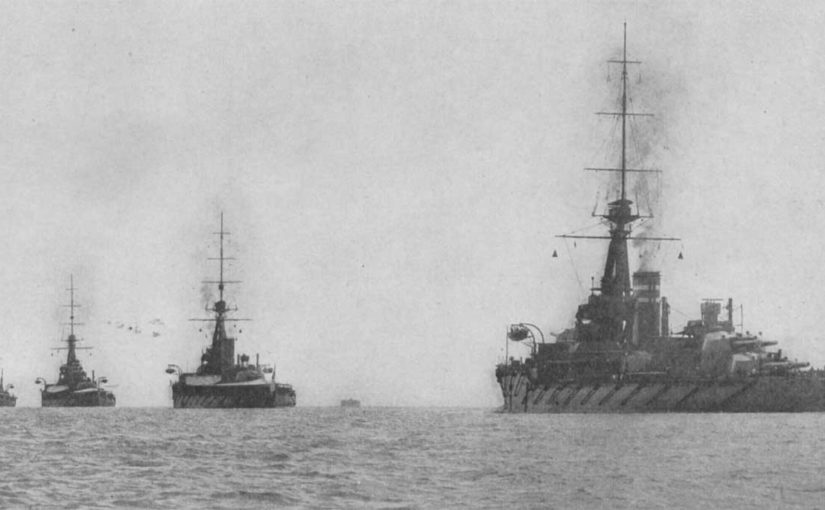
This could help explain why the first proposals of a similar set of equations were originally offered by Navy men – J.V. Chase, Bradley A. Fiske, and Ambroise Baudry. At sea, there is a predominance of attrition over manoeuvre: as Wayne P. Hughes points out in his classic reference work Fleet Tactics and Coastal Combat, “Forces at sea are not broken by encirclement; they are broken by destruction”. An attrition model may never take us beyond a mere casualty count in a land battle, but in the realm of naval action it might be just good enough.

There are other factors that make the sea an ideal testing environment for the practitioner of Operational Research. Hughes continues:

“The potential to effect this concentration [of force] is greater at sea than on land. At sea there is no high ground, no river barrier, no concealment in forests that requires what is often used as a rule of thumb on land, a 3:1 preponderance of force to attack a prepared position […]. Sun, wind, and sea state all affect naval tactics, but not to the extent that terrain affects ground combat.”

He concludes that the main objective of naval tactics throughout history has been the successful attack, and that is achieved by concentration of firepower – Lanchester would have agreed. Although today we still refer to the Square Law as Lanchester’s creation and by his name, it can be argued that the models created by Chase, Fiske and Baudry not only predate it, but are also more fortunate in their application from their conception, being better adjusted to the reality of war at sea.

THE MODEL

As presented in 1902, Lieutenant J.V. Chase’s own approach to the Square Law made the following assumptions, very similar to what Lanchester would postulate a decade later:

• When averaged out, shell fire from a fleet can be considered a continuous stream, rather than a series of individual projectiles.
• The two opposing fleets (let us call them Blue and Red) participating in the action are homogeneous: all ships in the Blue fleet are identical, and so are all ships in the Red fleet.
• The fighting power of a given ship is constant: it is unaffected by range, target aspect, spotting effectiveness, or morale.
• All ships in the fleet are able to fire at all ships in the opposing fleet, and no shots are wasted on a target that is already out of action.

The variables that describe the encounter are:

• The fleets engaged each have a number of ships, which we will refer to as A and B respectively.
• Ships have a “fighting power”, which we define as the number of accurate shots each of them can fire in a given unit of time. All ships in a fleet are assumed to have the same fighting power. We refer to the fighting power of Blue’s ships as α, and that of Red’s ships as β.

Finally, and as the main deviation from Lanchester’s formulation,

• Ships are also defined by their “staying power”: the number of shots they can withstand before being taken out of action. Again, all ships in a fleet are expected to be identical in this regard. We write the staying power of Blue’s ships as a, and that of Red’s as b.

It is worth mentioning that ships are, in this model, not necessarily taken out of action one by one: one intact ship is equal in every way to two ships that are halfway out of action. For this, we will refer to the results of Chase’s equations as the “equivalent” number of surviving ships, which represents the remaining combined combat strength of the fleet rather than an exact number of vessels.

The mathematical formulation, as presented by Wayne P. Hughes in The value of warship attributes in missile combat (1992) would look like this:

Where A and B are the number of ships in the Blue and Red fleets, α and β their fighting power, and a and b their staying power.

The state equations for a given time, obtained by integration:

A “square law” much in the spirit of Lanchester’s, and an identical attrition process being described. The only new factor, from a mathematical perspective, is the notion of “staying power”.

This difference might seem small at first (a mere denominator) but it is invaluable in practice: the model lets the practitioner explore the relative values of offence and defence, which in this formulation affect the end result equally, all else being the same. Chase himself, in a 1921 retrospective on his work, reflected:

“Having certain definite quantities of the various materials the question of ship design [is], …in the simplest form: “Shall we construct from these materials one ship or two ships?”…if we decide to build one ship instead of two, this single ship must be twice as strong offensively and twice as strong defensively as one of the two ships.”

History has taught us that fighting ships are susceptible to catastrophic damage; a torpedo strike, a bomb exploding below decks, or even a really unfortunate shell hit can take a well-armoured vessel out of action. This should make it abundantly clear that a ship twice the displacement of another is not necessarily twice as strong defensively. A design trend towards smaller vessels would seem mathematically reasonable.

As for the value of the concentration of firepower, let us run the experiment Chase proposed in the same retrospective we mentioned earlier.

A PRACTICAL CASE

Say we have two opposing fleets, both identical in every aspect.

Each has eight ships of comparable power; for the sake of our example, let us say all of them can fire on average 0.2 accurate shots per time increment, and all of them can take, say, twelve shots before they are disabled.

Of course, two such fleets (with identical combat strength and staying power) would eventually annihilate each other if they attacked at the same time and neither retreated.

Instead, let fleet Blue manoeuvre in such a way that one ship of fleet Red is masked and unable to fire. The contest is now temporarily eight ships versus seven – an apparently small imbalance. We apply the equations and plot the strength of both fleets as a function of time:

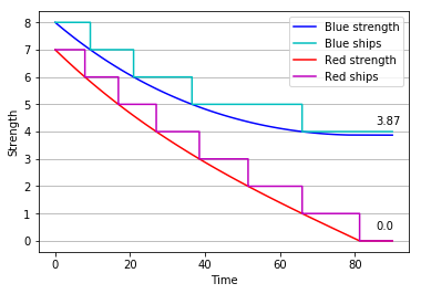
Predictably, the larger fleet wins this first phase of the engagement. We might find it more surprising that it does so by a comfortable margin, with the equivalent of 3.87 ships still in the fight – almost one half of the fleet’s original strength. These could now engage the lone remaining hostile ship, as shown below:

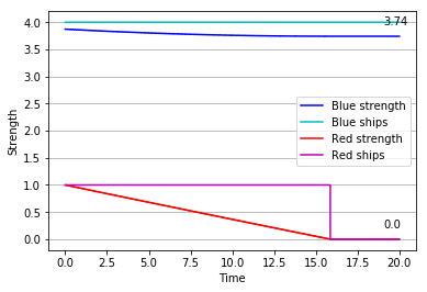
The last ship of fleet Red is eliminated with minimum damage to Blue – now at the equivalent of 3.74 battle-ready ships.

And so, a minor alteration in the initial conditions of the action grants fleet Blue a decisive victory, preserving almost half of its original force.

LESSONS

Chase’s model is a testament to the importance of concentration: the side engaging the fewest enemies while bringing the most guns to bear can expect to win, and manoeuvre should aim to secure this advantage. This much should be evident from our earlier example.

It also makes a compelling argument for the desirability of smaller ships. With offensive power and staying power having equal weight, the latter simply cannot be relied upon; the effects of enemy fire are difficult to quantify, and the possibility of catastrophic damage poses a great risk to any fleet concentrating its resources.

However, and perhaps more importantly, it shows how the shortcomings of attrition models are less conspicuous in the setting of naval warfare than they are on land; context matters.

GitHub

The Python implementations of the models used in this article for plotting simulated combat results can be found in the author’s GitHub page.

Further reading

1. Wayne P. Hughes – Fleet Tactics and Coastal Combat
2. Wayne P. Hughes –  The Value of Warship Attributes in Missile Combat
3. James G. Taylor – Lanchester-type Models of Warfare, Vol. I